Epic Games distributes a project called “Content Examples,” which is a collection of various sample projects showcasing different features of Unreal Engine. Since UE4.26, there is a map called Niagara Advanced.
This map contains a wealth of useful samples, including examples of new Niagara features and practical applications. Upon reviewing the implementations, there’s a lot to learn.
This article will break down these samples into multiple parts for detailed explanations.

By the way, Content Examples can be downloaded from this link in Fab. Please note that the content may vary depending on the version of UE.
※Note: This blog is written based on UE4.27 Contents Example, so it might differ from the latest version in small details, but the concept itself explained here won’t change.
TLDR;)
- You can implement PBD in Niagara and simulate real-time rigid constraints, like a chain simulation.
- Since you can combine this with existing Niagara modules, you can easily add forces like gravity or random shaking.
Introduction
In this article, we will discuss an advanced application of the previously introduced Position-Based Dynamics (PBD) by explaining a sample of a chain simulation using PBD. This corresponds to the “2.4 Iterative Constraints” section in Niagara Advanced.
2.4 Iterative Constraints Explanation
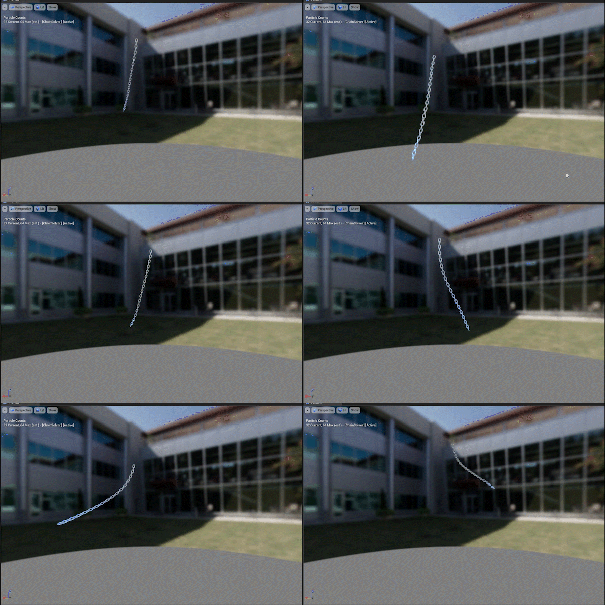
This sample demonstrates how to simulate the movement of a rigid constraint, like a chain, that does not stretch or shrink, using PBD.
In the video above, the chain is swaying back and forth, and each ring in the chain is represented by a Mesh Particle. The topmost particle has a programmed hard-coded movement, while the other particles are influenced by existing force modules and undergo position correction via PBD, ultimately giving the appearance of a connected chain moving.
Let’s take a look at the overall structure.
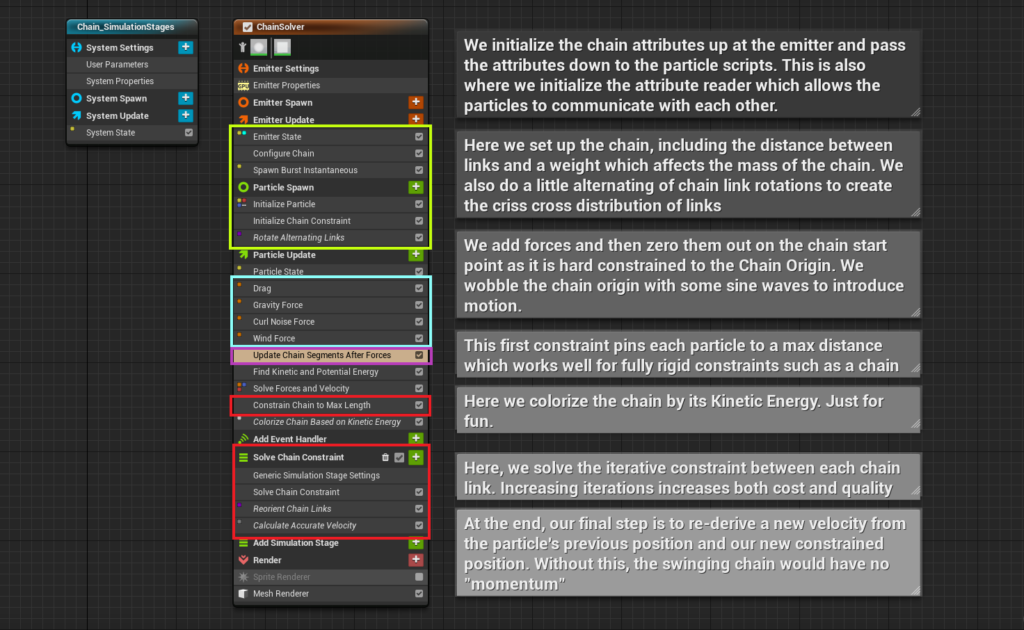
The setup consists of a single Emitter. Since we are using the Simulation Stage, it needs to be set to GPU simulation.
In the light green section, various parameters for the simulation are initialized, and initial positions and rotations for the particles are set.
In the light blue section, various forces are applied to the particles using existing modules.
The purple module is used to cancel forces and manually animate the position of the topmost particle.
Finally, in the red section, PBD is implemented. The main logic runs in the Simulation Stage, where the position correction is repeated 48 times per frame.
Let’s break this down in detail.
Chain Initialization
First, we configure the simulation parameters.
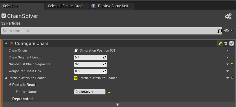
- Chain Origin: The starting point of the chain.
- Chain Segment Length: The distance between each ring in the chain (this is adjusted to match the size of the mesh).
- Number Of Chain Segments: The number of links in the chain (the number of particles spawned corresponds to this value).
- Weight Per Chain Link: The mass of each chain link (in this sample, this value is not used in the simulation).
Since PBD needs to know the positions of neighboring particles during the simulation, we also initialize the Particle Attribute Reader.
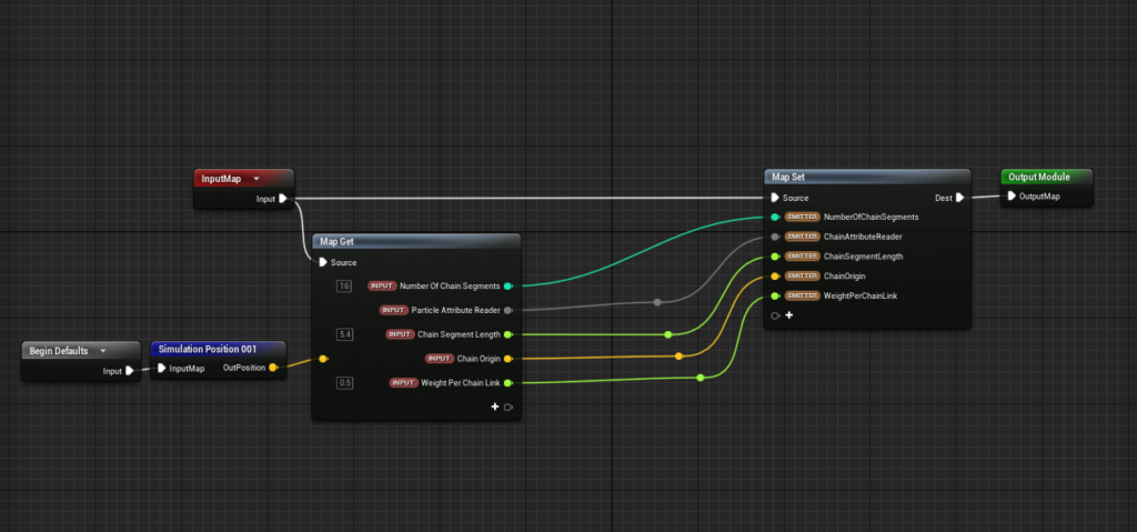
The Configure Chain module is a Scratch Pad Module that simply stores the initialized values in the Emitter’s attributes.
Next, Spawn Burst Instantaneous spawns the number of particles specified by Number Of Chain Segments all at once.
The Initialize Chain Constraint module initializes the positions and parameters of each particle representing the chain links.
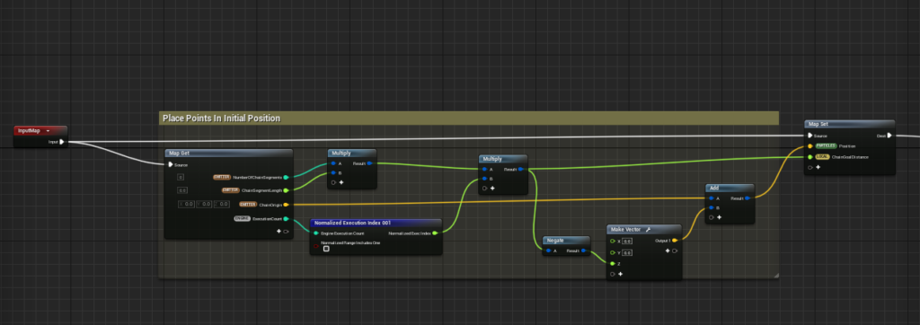
First, we initialize the positions of the particles. Using the values set in Configure Chain (starting point, number of particles, distance between particles), the particles are placed step-by-step in the negative Z direction.
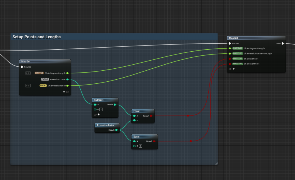
Next, we assign the following attributes to each particle:
- ChainSegmentLength: The initial length between particles (this will become the constraint in PBD).
- ChainGoalDistanceFromOrigin: The total length of the chain.
- ChainEndPoint: Flag indicating if the particle is at the end of the chain.
- ChainStartPoint: Flag indicating if the particle is at the start of the chain.
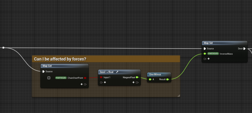
To prevent the start particle from being affected by forces, we create an InverseMass attribute. We set it to 0 for the start particle and 1 for the others.
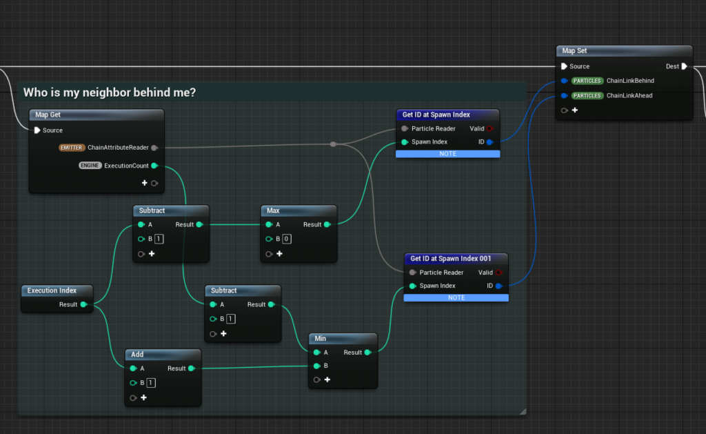
In PBD, each particle adjusts its position based on the distance from its neighboring particles. To facilitate this, we store the IDs of neighboring particles so that they can be referenced later in the Particle Attribute Reader.
Unlike Execution Index, particle IDs are unique even when new particles are generated, so using IDs is safer, especially when some particles are completely fixed in place.
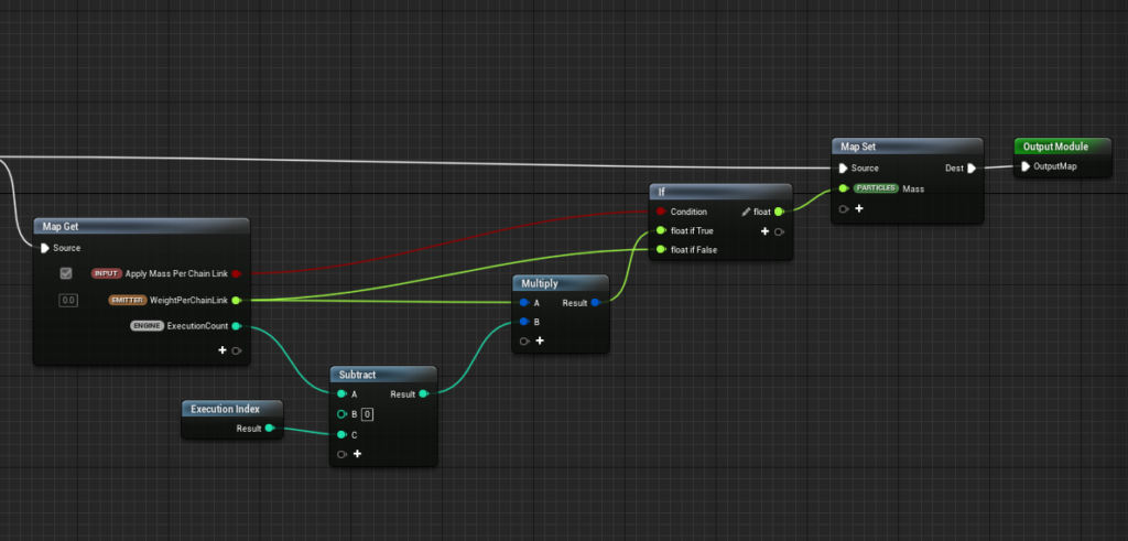
The mass value is stored in the Mass attribute, which will affect calculations when forces are applied in Niagara.
At the end of the chain initialization section, we also initialize the particle rotations. The goal is for the chain to rotate 90 degrees sequentially as it connects. We adjust the rotation based on whether the Execution Index is even or odd.
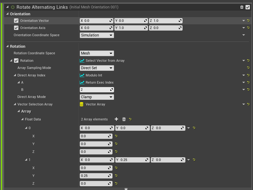
Force Configuration
The force part uses existing modules like Drag, Gravity Force, Curl Noise Force, and Wind Force, so we’ll skip the explanation here.
On the other hand, you can easily add more modules here to create different types of movements.
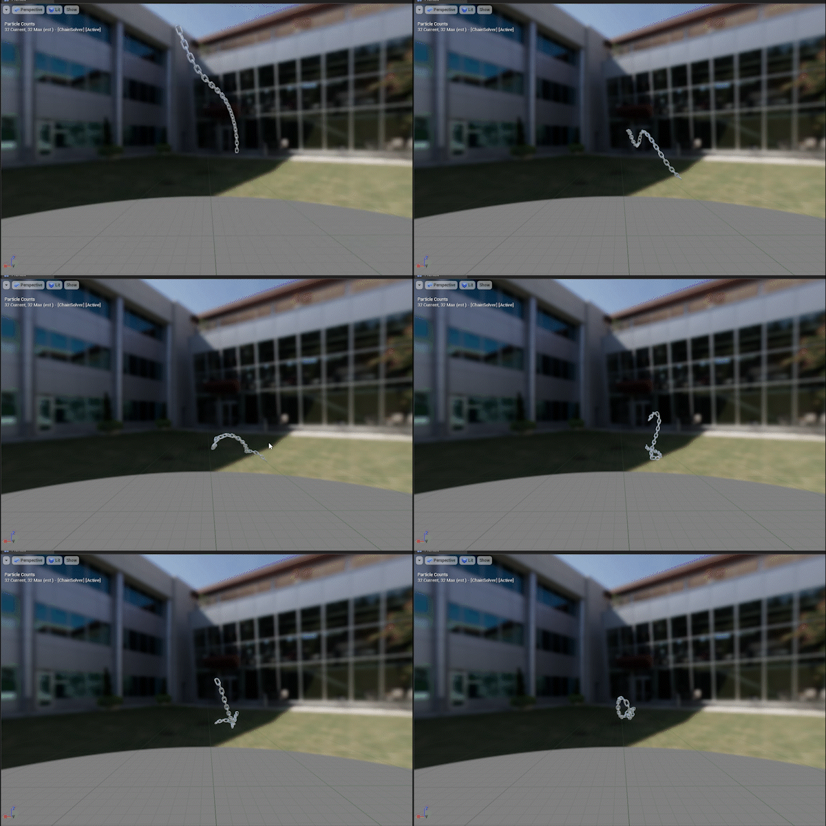
By the way, if you deactivate all the force modules, you will get the movement shown in the video above. As mentioned earlier, the start particle is hard-coded to move, and the remaining particles follow it through PBD.
Configuring the Start Particle’s Movement
The Update Chain Segments After Forces module cancels the forces applied to the start particle and applies its own movement. This is done using a Scratch Pad Module, so let’s take a look at its contents.
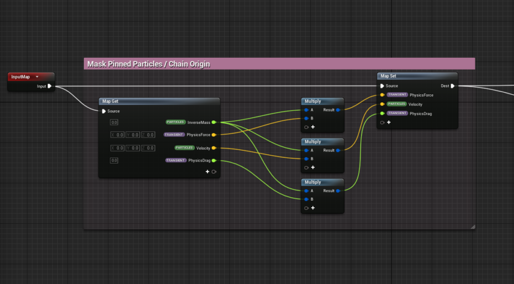
We multiply PhysicsForce, Velocity, and PhysicsDrag by InverseMass, so these values are 0 for the start particle.
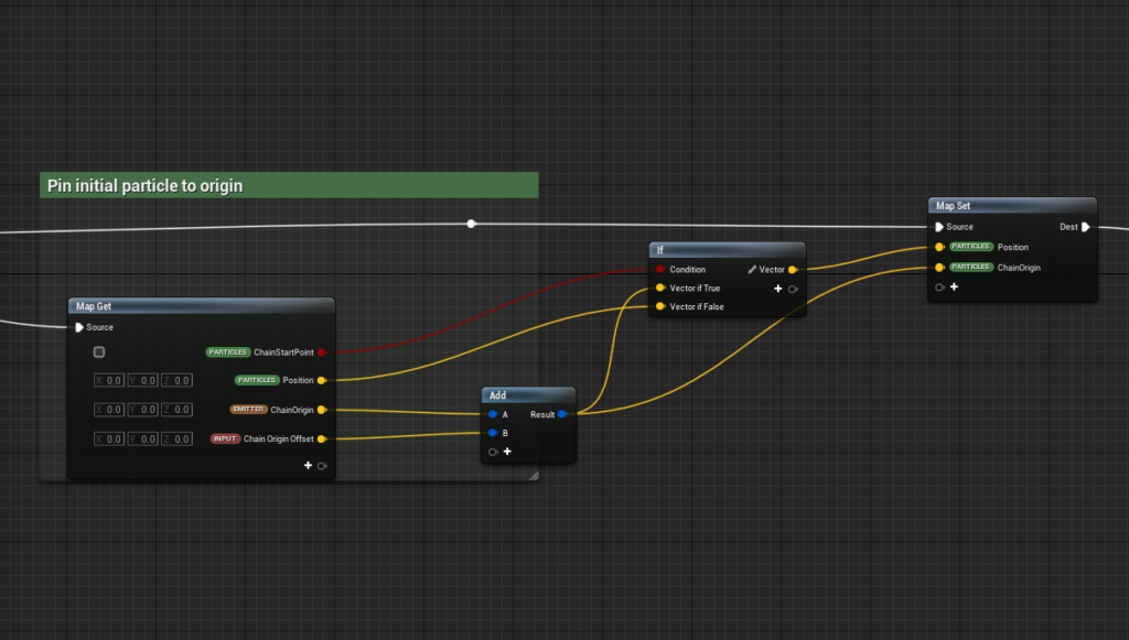
We then set the start particle’s position by adding an offset to ChainOrigin.
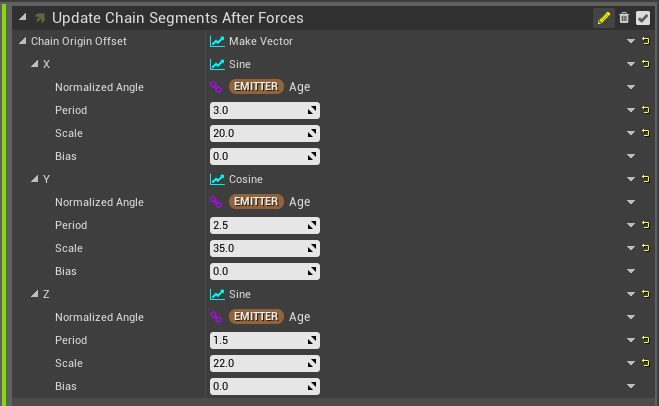
The offset moves in a sine curve along the x, y, and z axes over time, which animates the start particle’s movement.
If you disable the start particle’s animation, you’ll get the movement shown in the video below, where the start particle is fixed and the lower part of the chain sways under the influence of forces.
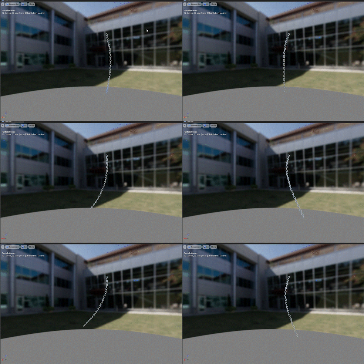
Coloring for Visualization
In the overview section, I didn’t mention the modules Find Kinetic and Potential Energy and Colorize Chain Based on Kinetic Energy (Color Module). These calculate the kinetic energy of the particles and use that value to color them, with the particles glowing blue based on the energy. This is a simple visualization and doesn’t require further explanation.
PBD Implementation
PBD does not calculate an object’s position from its velocity through mechanical equations. Instead, it adjusts the position iteratively to satisfy constraints. This method may lack some precision, but it allows for fast and robust simulations of complex movements, making it a popular choice for real-time applications.
In this example, the constraint is that the distance between particles cannot exceed a maximum value (the Chain Segment Length of 5.4). In the Particle Update stage, the particle’s position is adjusted to meet this constraint after external forces and velocity are applied.
The adjustment method is simple: calculate the distance to the neighboring particles, and if the distance exceeds the constraint, move the particle in that direction to correct the position.
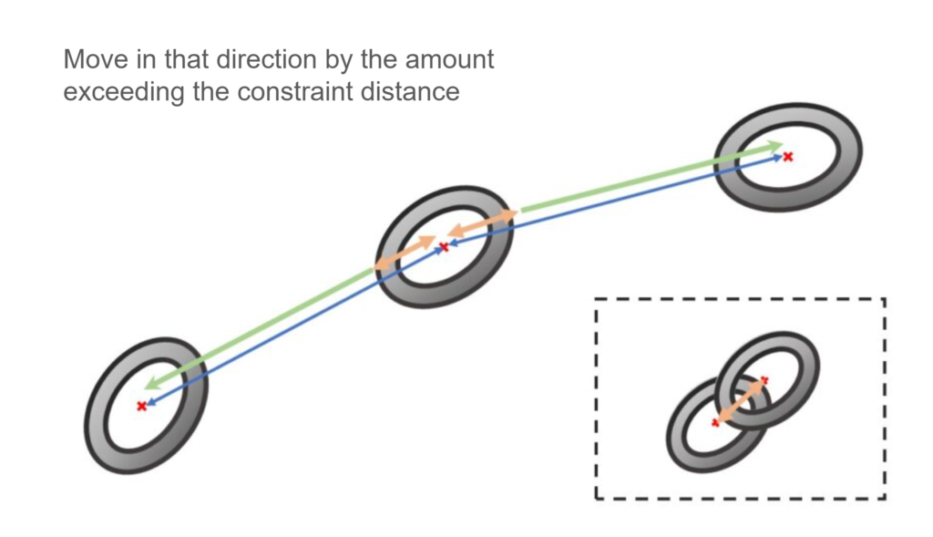
By performing this adjustment repeatedly, the system converges toward the optimal solution. In this example, the adjustment is performed 48 times per frame for each particle.
The more iterations you perform, the higher the accuracy, but naturally, the process will take more time.
Let’s take a look at the implementation.
There are four modules responsible for PBD within the Simulation Stage.
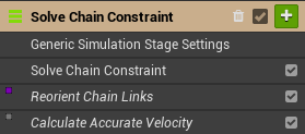
As shown below, the position adjustment process is repeated 48 times.
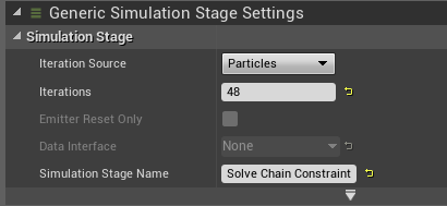
Solve Chain Constraint performs the position adjustment as described earlier.
Let’s take a closer look at the module’s implementation.
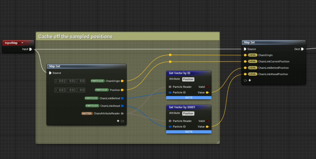
First, the Particle Attribute Reader retrieves the positions of the neighboring particles using the stored particle IDs.
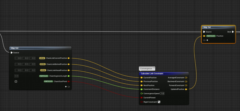
Then, the Calculate Link Constraint module script is passed the current position, neighboring particle positions, constraint distance, and a flag for pinning (whether the particle is fixed in place). The module outputs an UpdatedPosition that represents the adjusted position, which is then stored in the Position Attributes.
The Pinned flag ensures that the start particle’s position doesn’t change, as it is not affected by position adjustments.
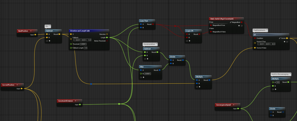
Inside the Calculate Link Constraint script, the direction vectors between particles are calculated. If the distance exceeds the constraint length, the particles are adjusted by the difference in distance in the direction of the vector.
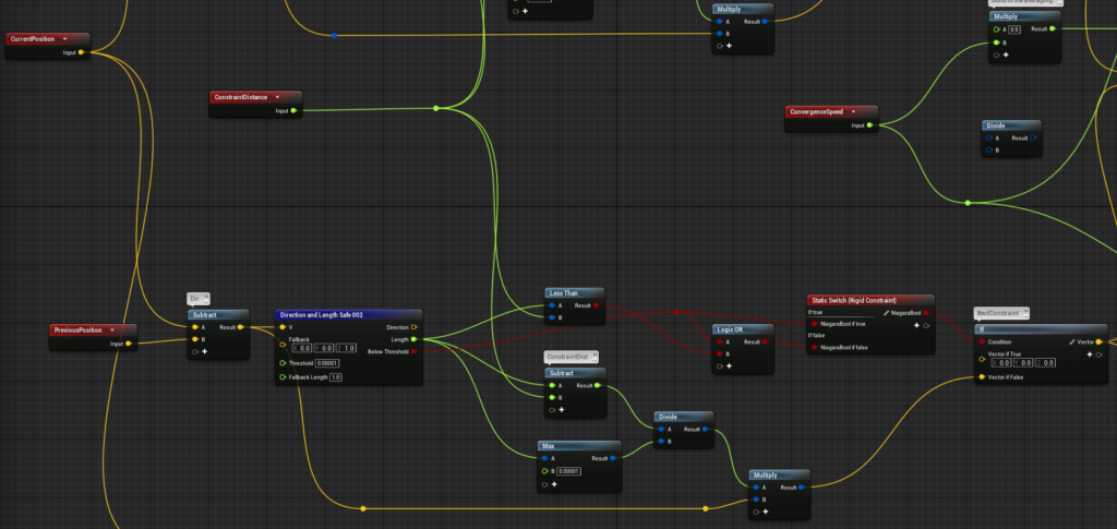
The calculation for the rear particles is done in the same way, and their vectors are determined.
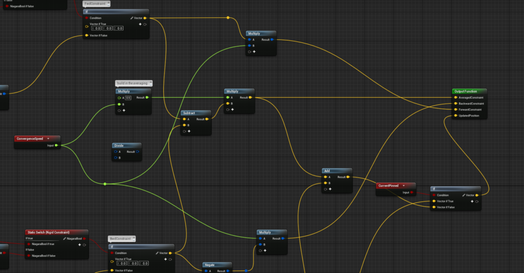
Then, the two vectors are added together and divided by 2. The resulting value is added to the particle’s original position, and the adjusted position is output as the UpdatedPosition. If the CurrentPinned flag is set to True, the position is not adjusted, and the original position is output instead.
This is how the position adjustment is calculated within the Calculate Link Constraint.
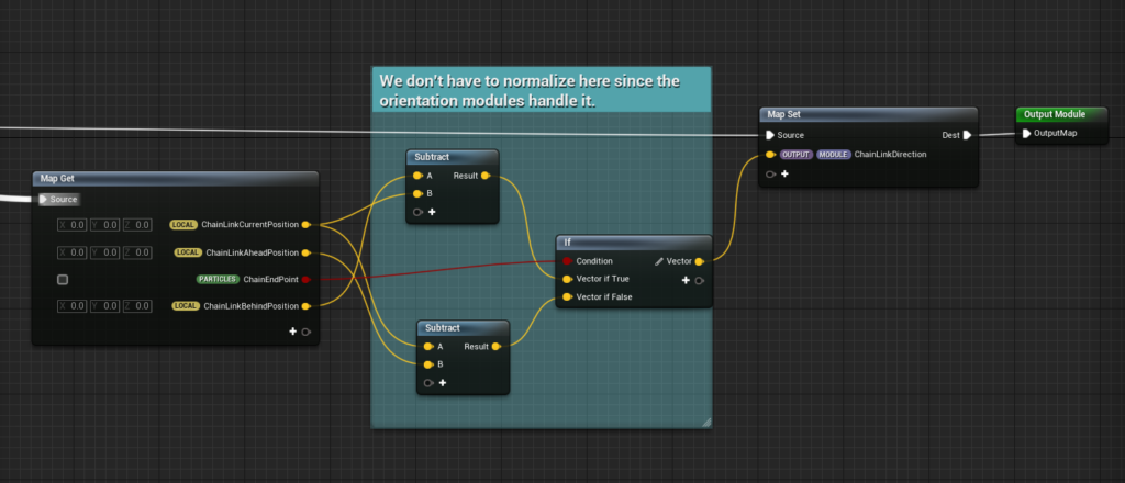
Next, to adjust the chain’s orientation, the vector to the previous particle is calculated and stored in ChainLinkDirection, which is then output. Since the end particle does not have a previous particle, the vector to the next particle is used instead.

Then, the Orient Mesh to Vector module (an existing module) takes the vector to the previous particle and inputs it into the Look At Direction. This ensures that the chain properly aligns in that direction.
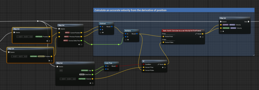
Finally, Calculate Accurate Velocity recalculates the velocity based on the adjusted position. The calculation is straightforward: subtract the previous frame’s position from the updated position and divide by the delta time.
In PBD, instead of calculating velocity from position, we recalculate the position from velocity to avoid any discrepancies during the next frame’s update.
I briefly skipped over explaining the Constrain Chain to Max Length Scratch Pad module in the Particle Update stage. This module checks if any particles have moved too far from the chain’s origin (beyond the total chain length). If they have, the module brings them back within the allowable range before the PBD position adjustment occurs. Although this step is not strictly necessary for this sample, it helps the PBD adjustments converge more efficiently.
The implementation is based on the same Calculate Link Constraint script, but with slightly different parameters.
That concludes the explanation of “2.4 Iterative Constraints.”
Conclusion
I was personally surprised by how simple the logic is for creating realistic rigid constraint movement with PBD.
As for performance, this sample (32 particles × 48 iterations) takes about 1ms for the PBD calculations on an RTX 2080. In a game environment, this may vary based on the situation, but for video and similar applications, this should be more than sufficient.
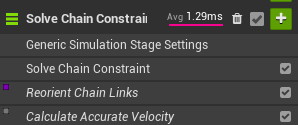
For instance, I tested with 100 particles and 60 iterations, and it took about 1–3ms. This is a reasonable load, but as always, it’s good to keep performance in mind.
One of the best things about this setup is that it can be combined with existing modules. It’s great for creating interactive simulations with collisions.
I tried creating a Mario Goomba character as an experiment, which I share in a separate article!
In conclusion, while using PBD for interactive simulations with collision still presents some challenges, I believe it can be incredibly useful in many other cases, and I look forward to seeing more examples of PBD in use.
Happy CG creation!


