Introduction
This time, I would like to explain “Normalize”, which is commonly used when doing somewhat technical things in visual effect creation.
※ By the way, the title is just an exaggeration as you know. I just wanted to give the title an interesting name…
Normalization itself is a mathematical term and is a concept that appears not only in visual effect creation and CG production but also in statistics and many other fields. The meaning of the term and the calculations involved can differ depending on the domain, so I don’t intend to go into strict technical details here.
Furthermore, normalizing is more about an approach or habit for improving efficiency and generalization rather than simply a piece of knowledge. I believe artists who do a little bit of math in tools like Shader, Niagara, or Houdini should definitely make this concept a part of their toolkit.
I’ll explain using examples from Unreal Engine, but the underlying concept doesn’t depend on the tools used, so even if you’re not using Unreal Engine, I encourage you to take a look!
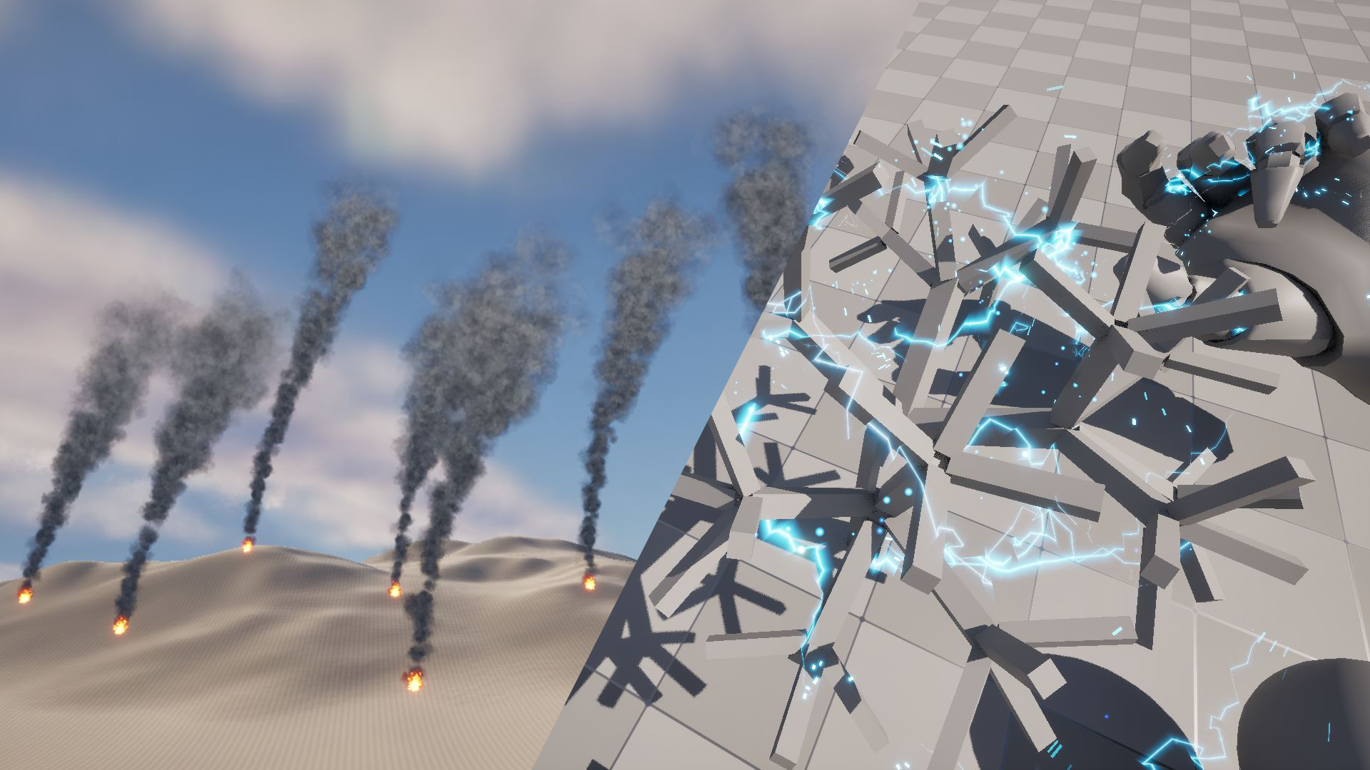
The data from the two examples mentioned below are available for sale, so feel free to check them out if you’re interested!
What is Normalize?
In CG production, when we talk about normalizing, there are generally two cases: normalizing a single value (float, scalar) and normalizing a vector (Vector2, 3, 4, etc.).
The core concept is the same in both cases, but for the sake of explanation and examples, it’s easier to separate them. This time, I will focus on normalizing a single value.
To put it simply, normalizing means “scaling the value range to 0~1.” It’s quite simple.
By the way, normalizing a vector means “making the vector’s length equal to 1.” It seems similar, doesn’t it?
To explain what it means to normalize a value into a 0~1 range, I’ll use Niagara’s “Normalized Age” as an example.
Normalized Age
As the name suggests, “Normalized Age” refers to the age that has been normalized. Age in this context means the number of seconds that have passed since a particle was created.
For example, if the lifetime of a particle is set to 2 seconds, the age will be the elapsed time since the particle’s birth, and it will disappear when it reaches 2 seconds. So, the age value will range from 0 to 2.

Now, what happens when you normalize this age? You scale the range from 0-2 into 0-1, so as shown in the figure, when the age is 1, the normalized value will be 0.5, and when the age is 2, the normalized value will be 1.

What Are the Benefits?
So, what benefits do we gain by normalizing the age to a 0~1 range? Let’s look at how Normalized Age is actually used.
In most cases, when creating effects, you might want to change attributes like color, size, or opacity according to the particle’s lifetime. For example, when fading out a particle, you might use a scale color node and set a curve on the alpha channel.
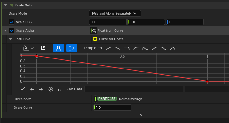
By default, the curve index is set to Normalized Age.
The curve reads as follows: the vertical axis represents the value returned (which would be the value assigned to Scale Alpha), and the horizontal axis represents the curve index (which is the Normalized Age). So, when the Normalized Age is 0, Scale Alpha is 1; when it’s 0.5, Scale Alpha is 0.5; and when it’s 1, Scale Alpha is 0.
As shown in the image above, this means that as the particle ages, the alpha gradually decreases, and when it dies, it reaches zero.
Now, if we set the particle’s lifetime to 2 seconds, we can recreate the same behavior by using Age in place of Normalized Age for the curve index, and setting the end point of the curve at 2 seconds, so that it reaches 0 when the lifetime is 2 seconds.
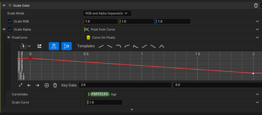
This will have the same effect as when using Normalized Age. However, this only works when the particle’s lifetime is exactly 2 seconds. For example, if the lifetime is set to 1 second, the particle will die when the alpha reaches 0.5, and if it’s set to 3 seconds, the alpha will reach 0 before the particle dies.
In reality, when emitting multiple particles, you often use random ranges to give particles different lifetimes. So, if you create a fade-out curve where alpha becomes 0 when age reaches 2 seconds, the fade-out behavior will change for particles with different lifetimes.
This is where Normalized Age comes in.
No matter what the lifetime of each particle is, the Normalized Age represents the particle’s life as a value between 0 and 1. If the lifetime is 2 seconds, 1 second, or 3.45 seconds, the Normalized Age will start at 0 when the particle is created, reach 0.5 at the halfway of its lifetime, and become 1 when the particle dies.
By using Normalized Age to set the curve, you can ensure that the fade-out occurs evenly for all particles, regardless of their lifetime.
Challenge Question!
How can we calculate Normalized Age? Think about it!
(The answer is at the bottom of this article)
Using Lerp with Normalized Age
You may not yet fully grasp the benefits of normalizing from the example of Normalized Age, so let’s take a look at a simple example where I combine Lerp and Normalize for even more useful applications.
I often use Lerp and Normalize together when I want to fine-tune the start and end values, or when I want to adjust the transition curve of the start and end values separately.
By the way, Lerp (Linear Interpolation) takes three inputs: A, B, and Alpha, and it returns a value between A and B, based on the ratio of Alpha.
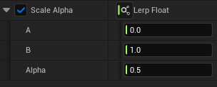
If Alpha is 0, Lerp returns the value of A (100% of A); if Alpha is 0.5, it returns the average of A and B (50% of A and 50% of B); and if Alpha is 1, it returns the value of B (100% of B). This is called linear interpolation.
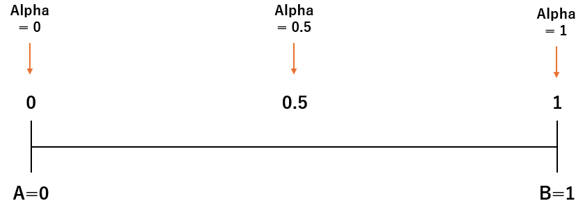
Now, when would you combine Lerp and Normalize? For example, I often use this approach when I want to apply power to a texture and control the fade-out by setting exponent (Exp) value dynamically through a Dynamic Parameter.
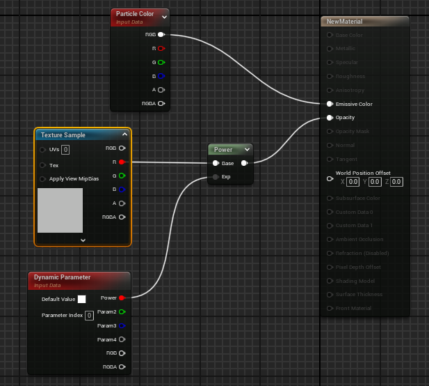
When applying power to a gradient texture, you can fade smoothly reflecting the texture’s appearance, but the exponent value that controls this fade-out often needs to be fine-tuned according to the desired look.
Normally, you might just use a curve to control the transition animation of the value and its easing, but the problem with this approach is that when you change the value, the curve’s easing also changes, requiring you to readjust the curve every time you change the value.
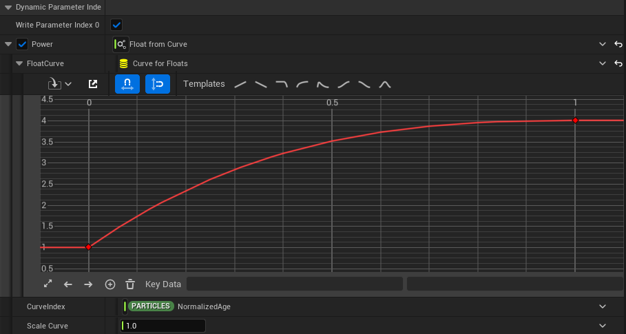
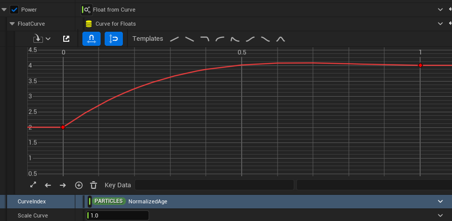
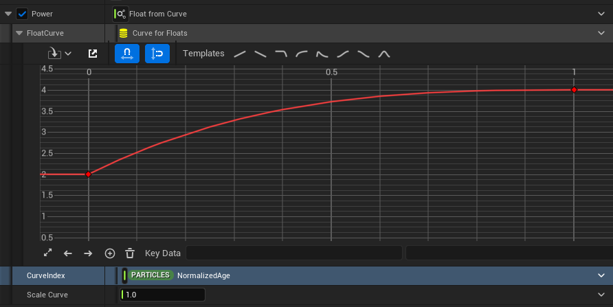
If you used just a curve, changing the start value would also change the curve’s easing, requiring you to adjust the curve every time you change a value, which is super inefficient.
By using Lerp, I set the start and end values as A and B, and use a curve to control the transition speed. This allows me to adjust the transition independently of the start and end values.
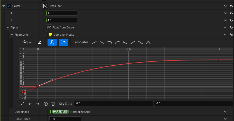
By separating the control of the start and end values from the control of the transition curve, I avoid having to adjust the curve every time I tweak the start or end value. This makes the process much more efficient.
Even though I haven’t directly used a normalized attribute here, the concept of normalization is still applied. Instead of adjusting the start and end values in the curve, I normalize the curve’s output to a 0–1 range and use Lerp to adjust the actual start and end values based on that.
This illustrates the point I made earlier about Normalize being more of a mindset or habit than just a technical knowledge.
I hope this gives you a better understanding of how Normalize can improve the workflow!
(Note: The Lerp example here does add a slight overhead in processing, so if performance is critical, you may want to optimize further. However, the overhead of Lerp isn’t dramatic, and the benefits of making adjustments more efficient often outweigh the extra cost.)
Example 1: Procedural High Smoke
After covering the finer points of Normalization, let’s look at a more fun example. This one involves using Normalization to create a smoke effect that rises high into the air.
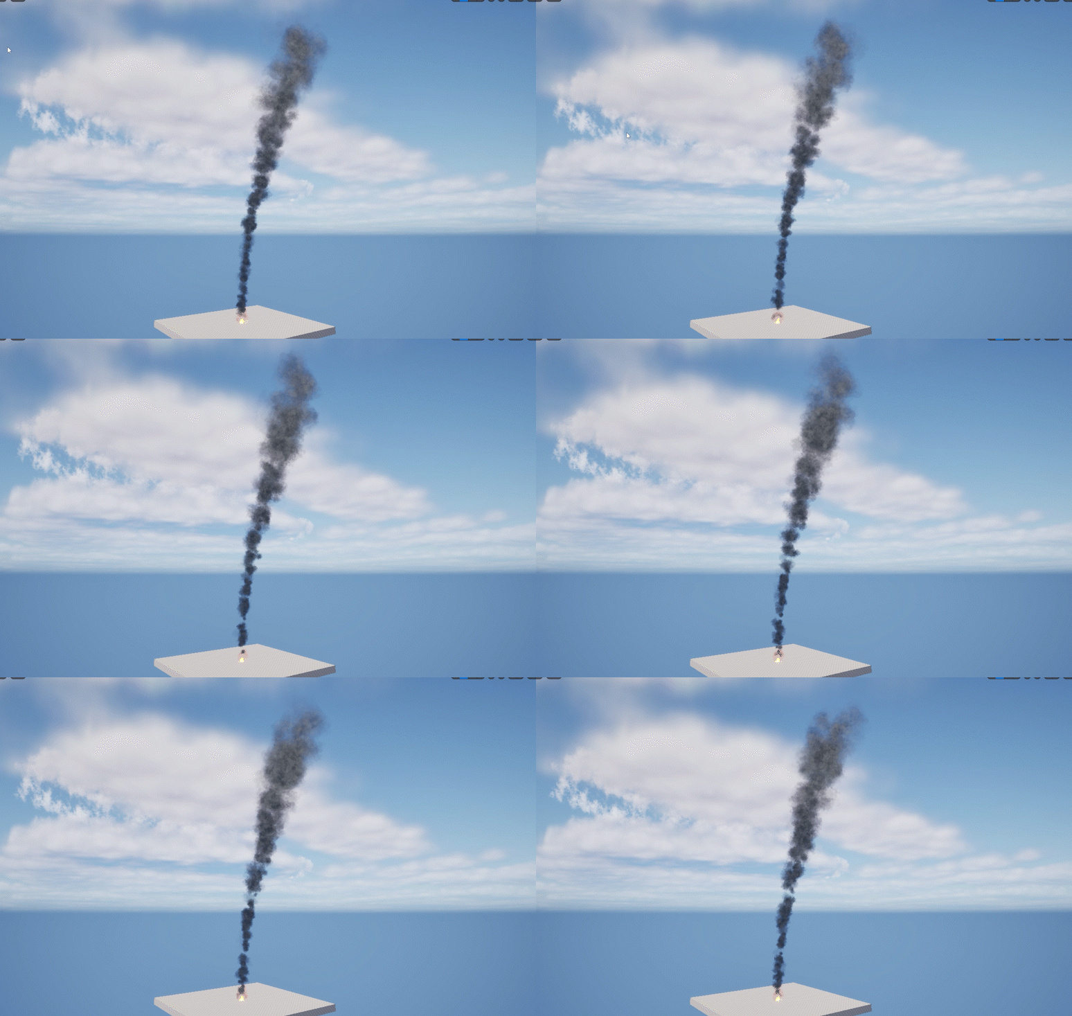
When creating background effects like this, how would you go about making smoke rise high into the air?
You might consider using Velocity or Force, but adjusting parameters this way can be tricky and time-consuming. It’s hard to get the ideal look, and it’s inefficient to wait for the particle to rise to check the result.
Instead, let’s reverse-engineer the physics: by understanding the visual behavior of the smoke at different heights, we can control the effect based on that.
Before jumping into the creation steps, let’s think about what the natural behavior of rising smoke looks like:
- Smoke coming from a fire rises quickly due to heat.
- As it rises and moves away from the fire, the smoke disperses and becomes lighter, influenced by wind.
- The smoke gets thinner and lighter as it rises higher into the air.
This behavior suggests that the appearance of smoke depends on its height. The higher it goes, the weaker the upward force becomes, and the more it spreads and thins out due to wind.
To achieve this look, you can adjust parameters like Velocity, Size, and Color based on the particle’s height. Let’s see how this works in practice.
Creation Steps
- Step 1: Decide the height range where you want the smoke to appear and spawn particles at that height.
- Step 2: Normalize the height of each particle and store that value in a new attribute,
NormalizedHeight. - Step 3: Create a curve,
HeightBias, based onNormalizedHeightto control the attributes like size and color. - Step 4: Use Lerp and the
HeightBiascurve to control particle attributes like Size, Color, and other properties based on height.
Normalizing the Height
First, let’s go over steps 1 and 2 of the creation process.
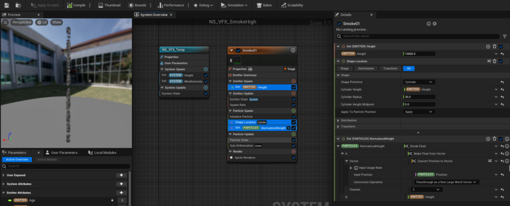
We create an attribute called “Height” in the Emitter and set it to 10,000.
By setting this to the “Cylinder Height” in the Shape Location (Cylinder), we can randomly generate particles between the z-values of 0 and 10,000.
Next, we create an attribute called “NormalizedHeight” in the Particle, and by dividing each particle’s position in the z-axis by the Height value, we can normalize the height. Simple, right?
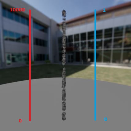
Creating a Curve Based on the Normalized Height
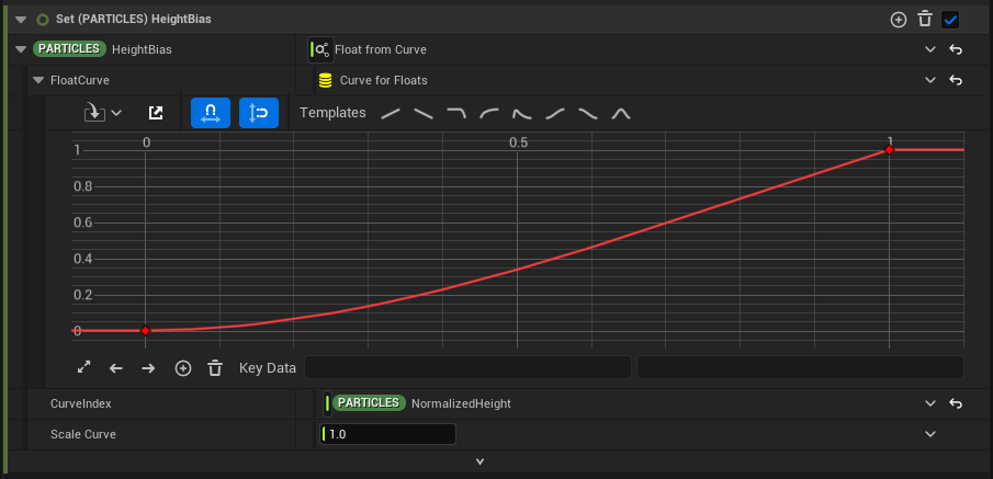
We create an attribute called “HeightBias” and set its value via a curve. By using NormalizedHeight in the CurveIndex, we can adjust how the value changes as the height increases.
It might be hard to grasp the meaning of this until we see how it is used, so let’s look at how the particles are affected by the wind and how they sway more as they move higher up.
The swaying behavior due to wind is expressed by simply changing the particle’s spawn position. In other words, particles that originally spawned in a straight line will be shifted according to the wind direction, with particles higher up moving further in the specified wind direction.
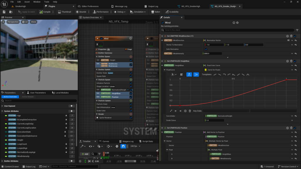
First, we create two parameters in the Emitter: “WindDirection” and “WindIntensity,” which define the wind’s direction and strength.
Then, we simply add the value of WindDirection × WindIntensity × HeightBias to the original position.
When NormalizedHeight is 0, HeightBias will be 0, and the value of WindDirection × WindIntensity × HeightBias will be 0, so the particle will not move from its original position.
On the other hand, when NormalizedHeight is 1, HeightBias will be 1, so the value of WindDirection × WindIntensity × HeightBias will equal WindDirection × WindIntensity. This means the particle will move in the direction of WindDirection by the amount set in WindIntensity.
In this way, the movement of particles can be controlled based on their NormalizedHeight. The degree of control can be fine-tuned using the curve for HeightBias.
For example, by setting the curve to a straight line, the particle movement will change linearly.

By adjusting the curve, you can control the movement based on the particle’s height. This is the purpose of setting the HeightBias.
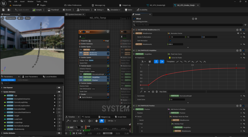
Using Height-Based Changes with HeightBias and Lerp
Now, let’s use the normalized height to affect other attributes. For instance, to simulate the spread of smoke that disperses more as it goes higher, we can spread the particles out in a spherical shape the higher they are, and also increase their size.
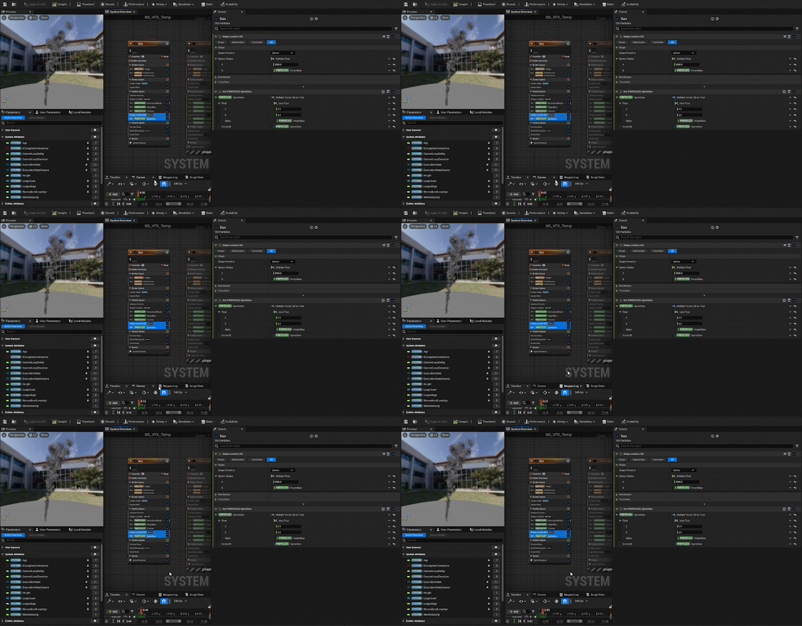
For attributes that should be zero when the height is zero, like the spread of particles, multiplying by HeightBias works fine. For example, the ShapeLocation (Sphere) “Sphere Radius” can be set to 2000 × HeightBias to increase the spread at higher altitudes while not affecting lower ones.
For the SpriteSize, since we don’t want the size to become zero, we use Lerp. We set HeightBias as the alpha value to control the size at both extremes: when HeightBias is 0 and when it is 1.
In the same way, we adjust other parameters:
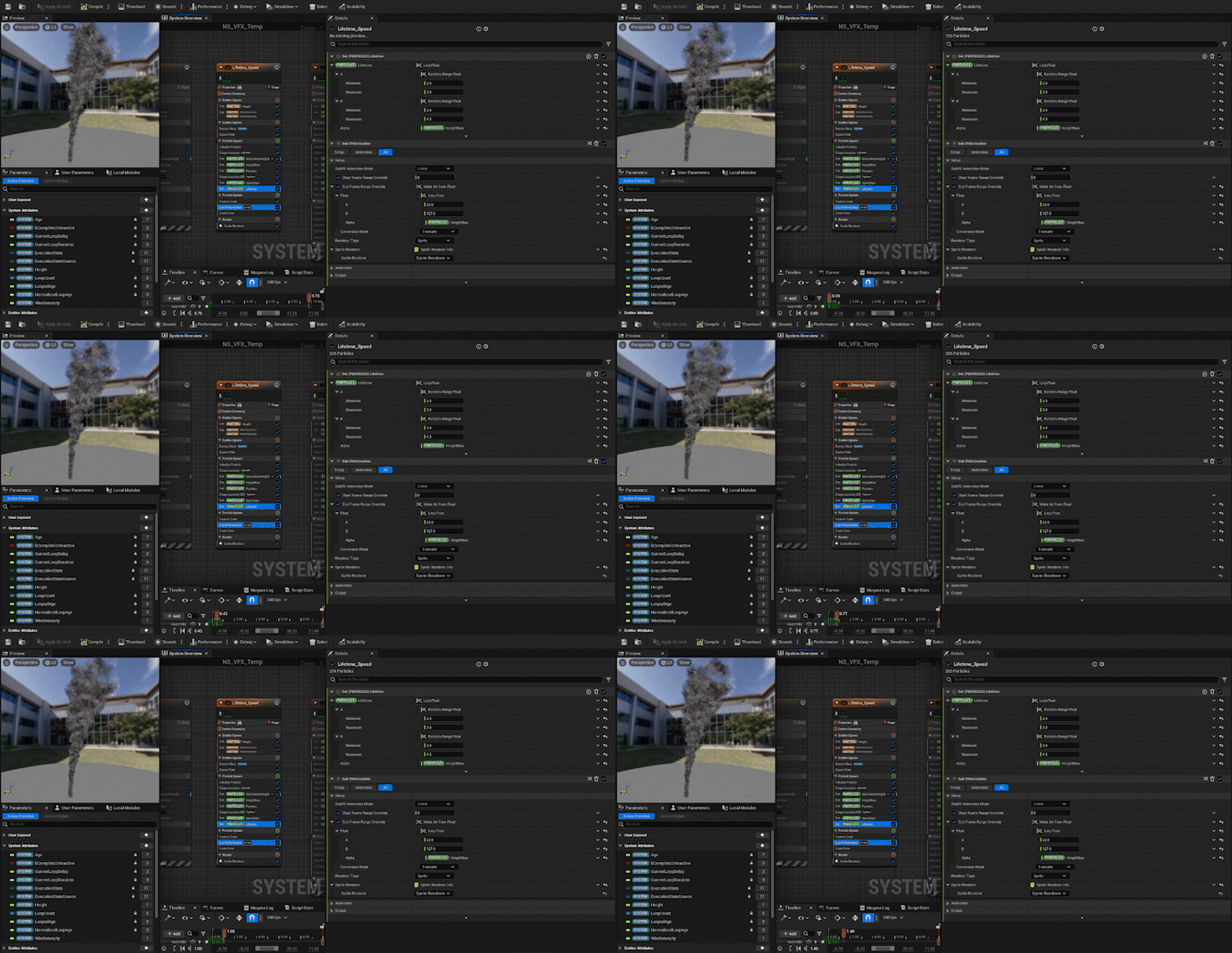
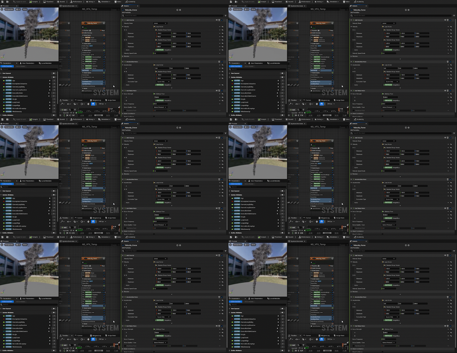
Curl Noise Force: The higher the particle, the stronger the force.
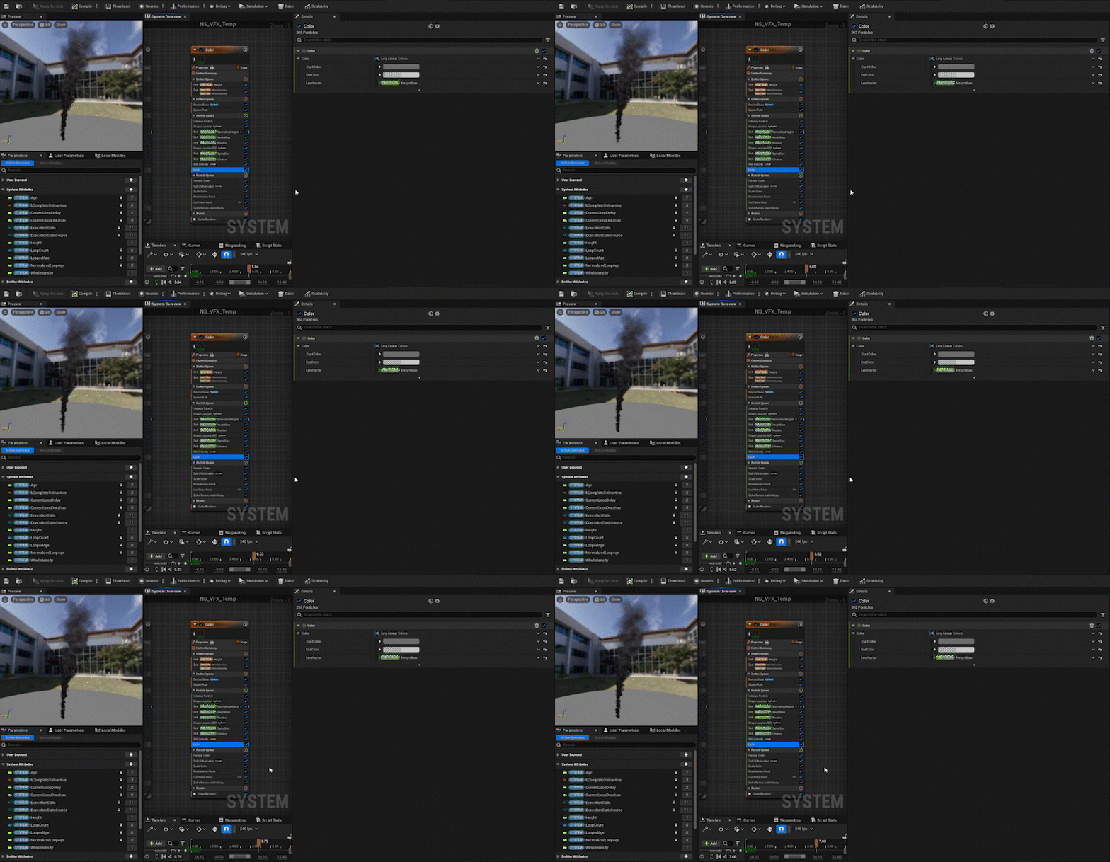
With these steps, we’ve created the basic framework for the rising smoke effect using normalization!
The Strength of Normalization
So far, we’ve seen that by using a normalized height value, controlling various attributes becomes much easier. But the real strength comes next.
When creating environment effects, you’ll often want to reuse the same effect multiple times across different areas. However, you don’t want all instances of the same effect to look exactly the same. To achieve variety, you can randomize various parameters.
For the rising smoke effect, for example, you’d want the height to vary within a certain range. And with normalization, you can do this easily! Not only that, but you don’t have to adjust other parts of the effect even when randomizing the height.
This is because, by using the normalized height to control the parameters, regardless of whether the height is 10,000, 800, or 15,000, the value of NormalizedHeight is always between 0 and 1.
So, with just a single effect, you can easily create variety by randomly varying the height. The beauty of normalization lies in that you can create these variations without worrying about the input values and adjust the subsequent processes accordingly.
By simply placing the effect in different locations, you can achieve the desired variety.
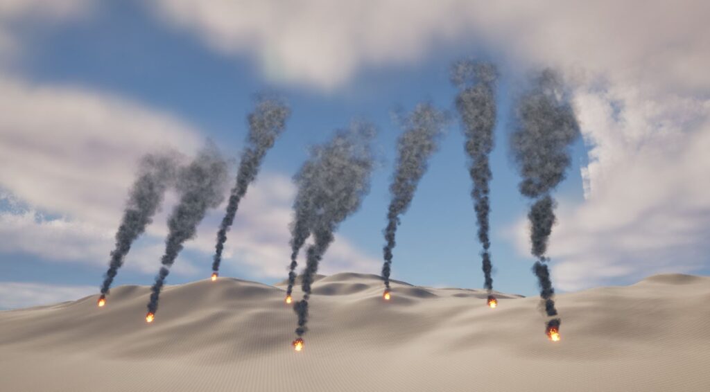
This is the real strength of normalization!
If you’re interested, you can find the data for this effect available for purchase at the link below:
Example 2: Procedural Lightning
Here’s the second example of using normalization: a procedural lightning effect. I’ll briefly explain the foundational mechanism behind this effect.
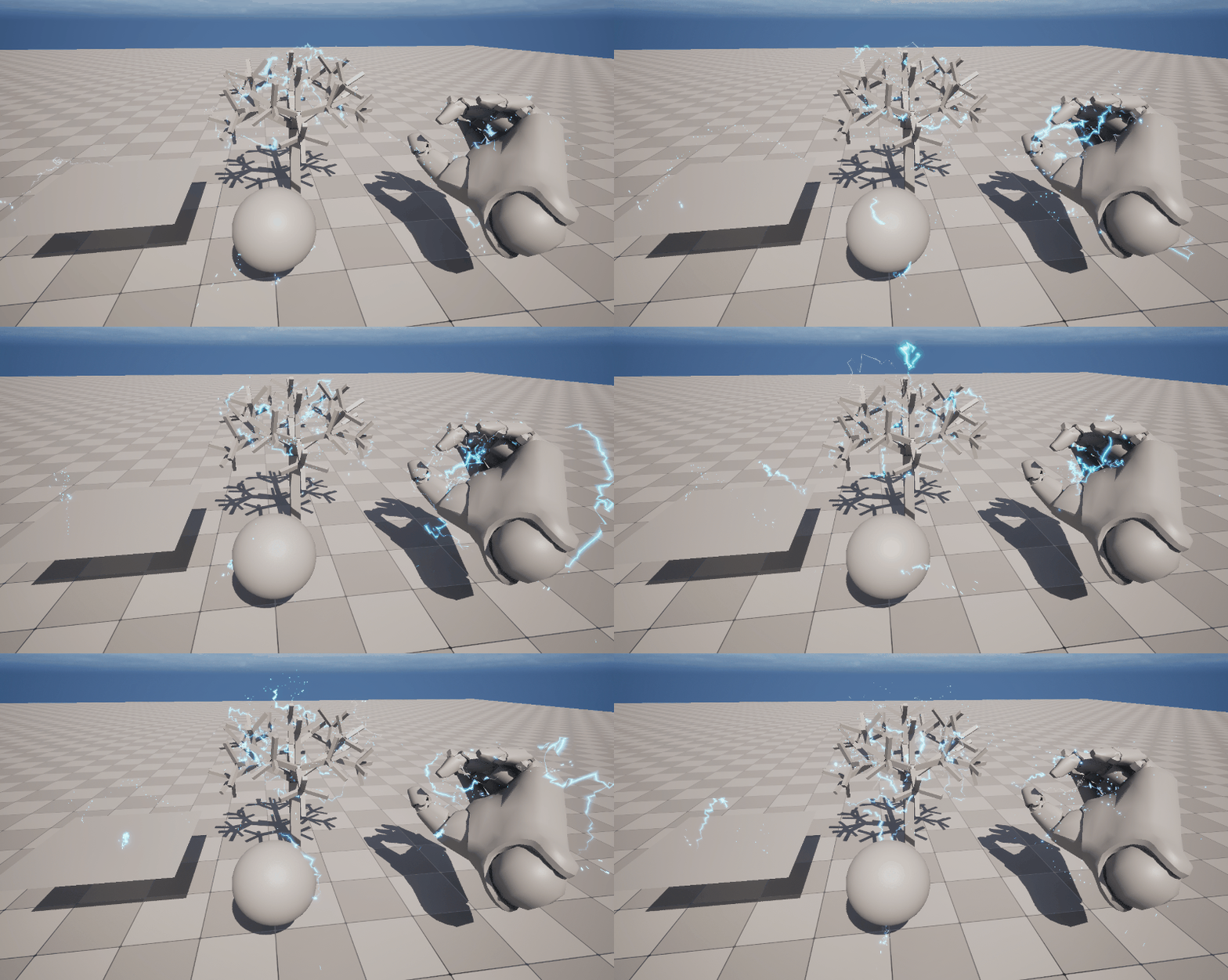
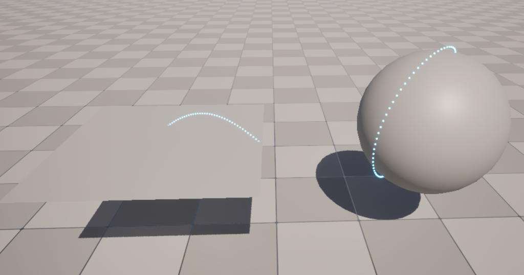
This lightning effect randomly selects two points on the surface of a Static Mesh and creates a lightning strike between those points. The great thing about this is that with a single effect, you can generate lightning for any Mesh automatically.
The fundamental mechanism is shown in the image below, where two points on the Mesh are connected with a Ribbon Renderer. Let’s walk through the details of that.
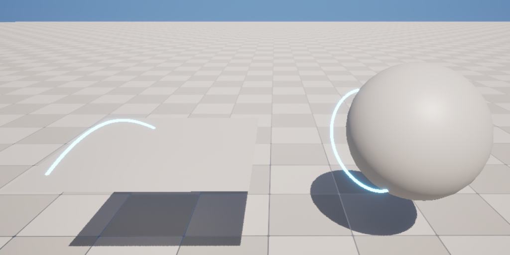
Overall Flow
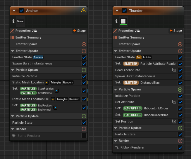
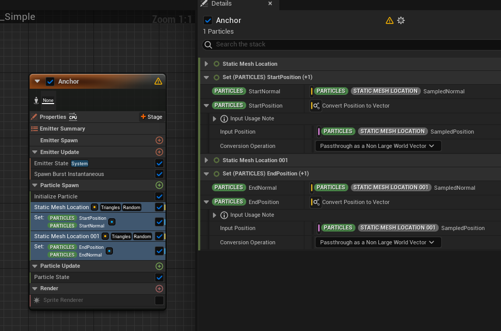
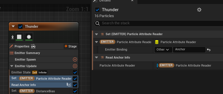
The basic setup consists of two Emitters. In the “Anchor” Emitter, the positions and normals of two points on the Static Mesh are retrieved, and the “Thunder” Emitter uses a Particle Attribute Reader to read and process this information.
The key part where normalization comes into play is when we use the Ribbon Renderer to connect the two points.
Ribbon (Particles) Placement
The Ribbon Renderer connects particles based on their RibbonLinkOrder, which defines the order in which the particles are connected. So, the key here is how to place the particles.
In the “Anchor” Emitter, we use the StaticMeshLocation to retrieve the position and normal of two points on the Mesh and create attributes for the start and end positions and normals.
These attributes are read by the Thunder Emitter via the Particle Attribute Reader.
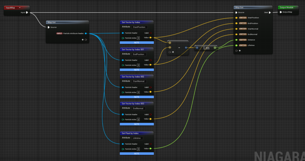
The “Read Anchor Info” is a Scratch Pad Module, and its purpose is simply to retrieve the Start/End Position and Start/End Normal from the Anchor and store them in the emitter’s attributes. Additionally, we also create a “Distance” attribute to store the distance between the start and end points.
We also wanted to specify the overall lifetime of the lightning, so we read the lifetime from the Anchor Emitter.
Now, let’s get into the particle placement process, starting with the explanation of the RibbonLinkOrder attribute.
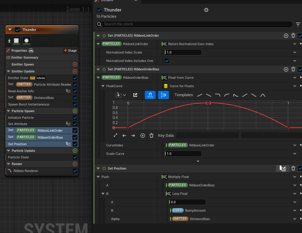
RibbonLinkOrder defines the order in which particles are connected by the Ribbon Renderer. The value is set between 0 and 1, and particles are connected based on their order, with lower values connected first.
Here, we set RibbonLinkOrder to use the normalized Exec Index value.
Normalization is involved here!
The Exec Index is the index assigned to each particle when it’s spawned (e.g., 0, 1, 2, etc., depending on the spawn order). Normalizing this Exec Index gives us a range of 0 to 1, which allows us to connect the particles in order of their spawn.
By normalizing the Exec Index, we can effectively connect the particles in sequence using RibbonLinkOrder.
Next, we’ll use this to actually place the Ribbon.
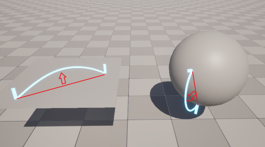
When placing the Ribbon, simply connecting the two points obtained from the Mesh with a straight line will cause the Ribbon to intersect with the Mesh. Therefore, we need to keep the two points on the Mesh fixed and adjust the placement to avoid the Ribbon intersecting with the Mesh, by “inflating” the area between them.
To do this, we create a curve from the Ribbon Link Order and set a coefficient that controls how much the Ribbon will inflate.
We create an attribute called RibbonOffsetBias, and set the CurveIndex to RibbonLinkOrder to create the curve. As shown in the image, we create a curve where the value is 0 at RibbonLinkOrder = 0 & 1 and 1 at RibbonLinkOrder = 0.5, resulting in a “mountain-shaped” curve. This way, the positions at both ends of the Ribbon stay fixed, and we can offset the Ribbon toward the center.
Using this coefficient for inflation, RibbonLinkOrder, and the Start/EndPosition and Start/EndNormal values obtained from the Mesh, we can now place the Ribbon. Here’s how we do it:

First, we linearly interpolate (Lerp) between the StartPosition and EndPosition using RibbonLinkOrder. This process alone will create a Ribbon that connects the Start and End Positions with a straight line.
Next, to apply the inflation, we use spherical linear interpolation (Slerp) between the StartNormal and EndNormal to determine the direction. We then multiply it by a value called Push to calculate the offset, and add that to the position calculated earlier, resulting in the final inflated position.
To clarify the difference between Lerp and Slerp: Lerp is linear interpolation, which is used when you want to connect two values along a straight line, while Slerp is spherical linear interpolation, which is used when you want to rotate between two directions (vectors).
In this case, to prevent the Ribbon from intersecting the Mesh, we inflate the Ribbon by rotating between the normal direction of the Mesh at the start point and the normal direction of the Mesh at the end point. This approach works well when using Slerp for the transition in RibbonLinkOrder.
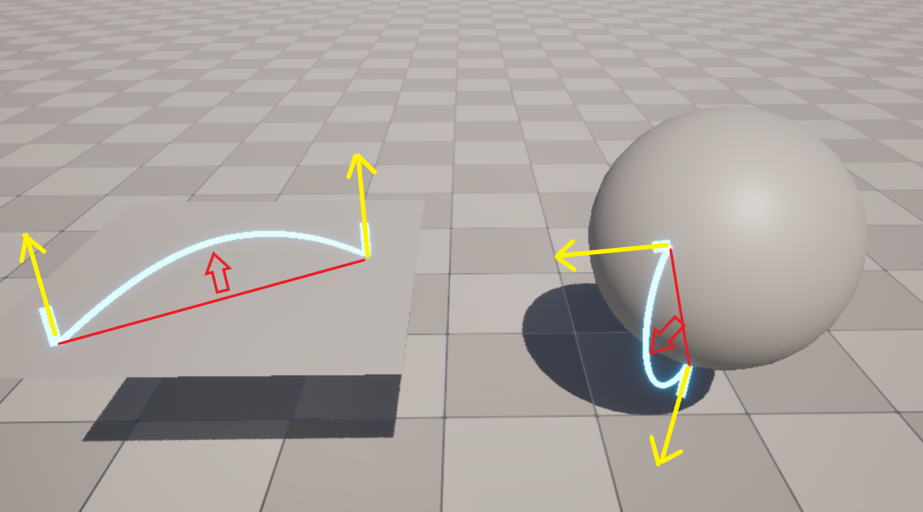
Finally, the amount of inflation controlled by the Push value is calculated by multiplying the RibbonOrderBias and the maximum offset value for the inflation.

With this method, we can create a Ribbon that connects any two points on a Mesh. This is the foundational mechanism of the procedural lightning effect.
Afterward, we can add some noise, animate the Ribbon, tweak shaders, and add particles to enhance the lightning effect, but I’ll skip those details for now.
Though I won’t go into full details here, the complete data for this effect is available for purchase at the following link if you’re interested.
Conclusion
Although this might have been a challenging topic for some artists, VFX artists are increasingly able to create complex effects with tools like Niagara, Houdini, and VFX Graph without relying on engineers. Understanding mathematical concepts like normalization can be incredibly helpful when exploring these tools and creating even more compelling visual effects.
Normalization is just one of many tools that can unlock new creative possibilities. If you’re interested, vector normalization is another important concept commonly used in VFX, and diving into it can be very rewarding!
(For those who want to check out the answer to the challenge problem, it’s: Normalized Age = Age / Lifetime.)
